1. Types of Errors
What is it? Errors occur when data bits are altered during transmission or storage due to noise, interference, or hardware faults. Understanding error types helps in designing appropriate detection and correction mechanisms.
Key Types:
- Single-Bit Error:
- Only one bit in the data flips (e.g.,
1010→1000). - Common in low-noise environments.
- Example: A cosmic ray flips a single bit in memory.
- Only one bit in the data flips (e.g.,
- Burst Error:
- A sequence of consecutive bits is corrupted.
- Length of the burst is the number of bits from the first to the last error (e.g.,
101010→100110, burst length = 3). - Common in noisy channels like wireless communication.
- Multiple-Bit Error (Non-Burst):
- Multiple bits are corrupted, but not consecutively (e.g.,
101010→111100, errors in positions 2 and 5). - Less common but harder to detect/correct.
- Multiple bits are corrupted, but not consecutively (e.g.,
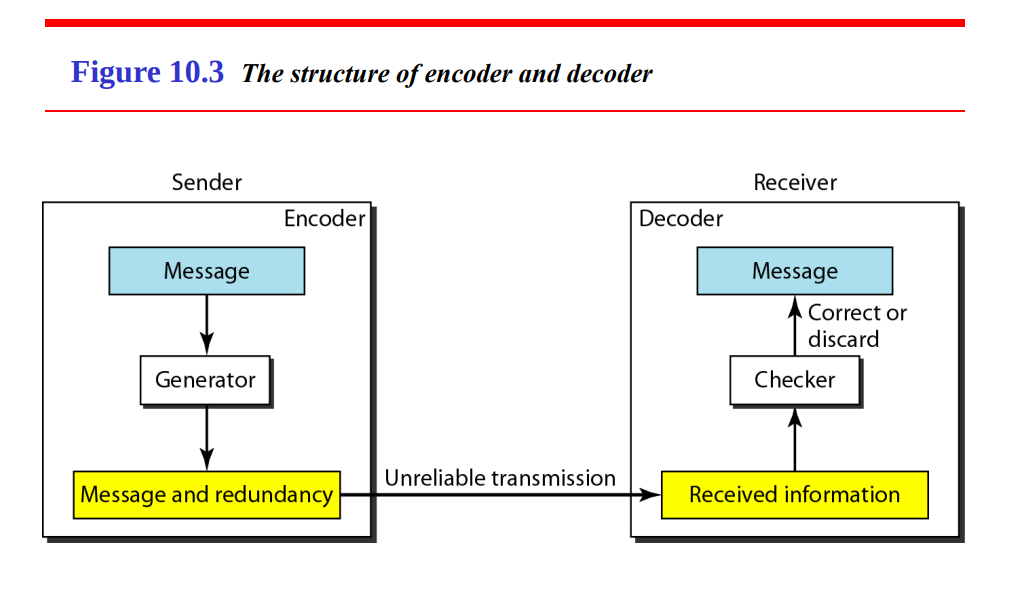
Sender Side (Encoder)
The sender’s job is to encode the original message with redundancy to enable error detection or correction at the receiver.
-
Message:
- This is the original data the sender wants to transmit (e.g., a binary string like
1011). - It consists of
kbits of actual information.
- This is the original data the sender wants to transmit (e.g., a binary string like
-
Generator:
- The generator is the component (or algorithm) that adds redundancy to the message.
- It takes the original message and appends redundant bits to create a codeword.
- How it Works:
- Redundancy can be added using techniques like parity bits, Hamming Code, or CRC.
- For example, in CRC, the generator polynomial (e.g.,
x^3 + 1) is used to compute a check value that’s appended to the message.
- Output: A codeword consisting of the original message plus redundant bits.
- If the message is
kbits, andrredundant bits are added, the codeword isn = k + rbits.
- If the message is
-
Message and Redundancy:
- This block represents the final codeword ready for transmission.
- It includes:
- The original message (
kbits). - Redundant bits (
rbits) for error detection/correction.
- The original message (
- Example: For a message
1101with a 3-bit CRC100, the transmitted codeword is1101100.
-
Unreliable Transmission:
- The codeword is sent over an unreliable channel (e.g., a noisy wireless link).
- Errors may occur during transmission (e.g.,
1101100might become1100100if a bit flips).
Receiver Side (Decoder)
The receiver’s job is to process the received data, detect any errors, and either correct them or discard the data if errors are uncorrectable.
-
Received Information:
- This is the data the receiver gets after transmission.
- It may be identical to the sent codeword (
message + redundancy) or may contain errors due to the unreliable channel. - Example: Sent
1101100, but received1100100(bit 4 flipped).
-
Checker:
- The checker is the component that examines the received codeword to detect errors.
- How it Works:
- It uses the redundant bits to verify the integrity of the data.
- Depending on the technique:
- Error Detection: Determines if an error exists (e.g., CRC checks if the remainder is 0).
- Error Correction: Identifies and fixes errors (e.g., Hamming Code uses a syndrome to locate the error).
- Examples:
- CRC: Divide the received codeword by the generator polynomial. If the remainder is 0, no error; otherwise, an error is detected.
- Hamming Code: Compute a syndrome to detect and correct a single-bit error.
- Outcome:
- If no errors are detected, the message is accepted.
- If errors are detected:
- For error correction: Fix the error (e.g., Hamming Code flips the erroneous bit).
- For error detection only: Discard the data or request retransmission (e.g., CRC in Ethernet).
-
Correct or Discard:
- This step indicates the action taken by the decoder:
- Correct: If the system supports error correction (e.g., Hamming Code), the checker fixes the error, and the original message is recovered.
- Discard: If the system only supports error detection (e.g., CRC), or if the errors are uncorrectable (e.g., too many bit flips for Hamming Code), the data is discarded.
- In systems with retransmission (e.g., ARQ protocols), the receiver may request the sender to retransmit the data.
- This step indicates the action taken by the decoder:
-
Message:
- This is the final output at the receiver.
- If the checker successfully detects and corrects errors (or if no errors occurred), this is the original message (e.g.,
1101). - If the data is discarded, no message is output, and the receiver may take further action (e.g., request retransmission).
What is Block Coding?
Block coding is a method used to add redundancy to digital data to enable error detection or correction. It works by dividing the data into fixed-size blocks and appending redundant bits to each block, creating a codeword that can be transmitted or stored reliably. The receiver uses these redundant bits to detect or correct errors introduced during transmission or storage.
Key Idea: Each block of data is treated independently, and redundancy ensures the receiver can identify or fix errors without needing to retransmit the data (in the case of correction).
How Block Coding Works
-
Data Division:
- The message (data to be sent) is divided into blocks of k bits. Each block is processed independently.
- Example: A 16-bit message
1011001110101100might be split into four 4-bit blocks:1011,0011,1010,1100.
-
Adding Redundancy:
- For each k-bit block, r redundant bits are added to form an n-bit codeword, where
n = k + r. - These redundant bits are calculated based on the data bits using a specific coding scheme.
- The redundant bits enable the receiver to detect or correct errors.
- For each k-bit block, r redundant bits are added to form an n-bit codeword, where
-
Codeword:
- The resulting n-bit codeword consists of the original k data bits plus the r redundant bits.
- Example: A 4-bit data block
1011with 1 parity bit (r = 1) becomes a 5-bit codeword10111(even parity).
-
Transmission:
- The codeword is transmitted over a communication channel or stored in a medium (e.g., disk, memory).
-
Receiver Processing:
- The receiver checks the received codeword using the redundant bits:
- Error Detection: Verifies if the codeword is valid (e.g., parity check fails if the number of 1s is odd).
- Error Correction: Identifies and corrects errors (e.g., Hamming Code locates and fixes a single-bit error).
- The receiver checks the received codeword using the redundant bits:
Key Properties of Block Coding
-
Code Rate:
- Defined as
k/n, the ratio of data bits to total bits in the codeword. - A higher code rate (closer to 1) means less redundancy but weaker error handling.
- Example: For
k = 4,r = 3,n = 7, the code rate is4/7 ≈ 0.57.
- Defined as
-
Systematic vs. Non-Systematic:
- Systematic: The codeword contains the original data bits followed by the redundant bits (e.g.,
1011+ parity1=10111). - Non-Systematic: The codeword is a transformed version of the data, not directly containing the original bits (less common).
- Systematic: The codeword contains the original data bits followed by the redundant bits (e.g.,
Advantages of Block Coding
- Reliability: Enables detection and correction of errors, ensuring data integrity.
- Simplicity: Fixed block size makes implementation straightforward (e.g., in hardware).
- Flexibility: Different block codes (e.g., Hamming, CRC) can be chosen based on the type of errors expected (single-bit vs. burst).
- No Feedback Required: For error correction, no retransmission is needed, unlike detection-only methods.
Limitations of Block Coding
- Overhead: Adding redundant bits increases the data size, reducing the effective data rate.
- Limited Error Handling:
- Simple codes like parity can’t correct errors or detect all multi-bit errors.
- Hamming Code corrects only single-bit errors.
- Complexity: Advanced codes like Reed-Solomon require more computational resources for encoding/decoding.
- Fixed Block Size: May not be efficient for variable-length data streams (unlike convolutional coding).
Applications of Block Coding
- Communication Systems:
- Hamming Codes: Used in memory systems (e.g., ECC RAM) to correct single-bit errors.
- CRC: Used in Ethernet, Wi-Fi, and USB to detect burst errors.
- Storage Systems:
- Reed-Solomon: Used in CDs, DVDs, and SSDs to correct errors due to scratches or defects.
- Networking:
- CRC in packet headers (e.g., Ethernet frames) ensures data integrity.
- Space Communication:
- Block codes like Reed-Solomon are used in satellite and deep-space communication to handle high error rates.
Hamming Distance
The Hamming Distance between two codewords (or binary strings) of equal length is the number of positions at which their bits differ. It’s a metric used to quantify how “different” two codewords are, which directly impacts a code’s ability to detect and correct errors.
- Formal Definition: For two codewords
C1andC2of lengthn, the Hamming Distanced(C1, C2)is the number of bit positions whereC1[i] ≠ C2[i]. - Example:
C1 = 10110C2 = 10011- Compare bit by bit:
10110vs10011- Position 1:
1vs1→ Same - Position 2:
0vs0→ Same - Position 3:
1vs0→ Different - Position 4:
1vs1→ Same - Position 5:
0vs1→ Different
- Position 1:
- Hamming Distance = 2 (differ at positions 3 and 5).
Minimum Hamming Distance (d_min)
The Minimum Hamming Distance (d_min) of a code is the smallest Hamming Distance between any two distinct valid codewords in the code. It’s a critical property that determines the error-handling capability of the code.
- How to Calculate:
- List all valid codewords in the code.
- Compute the Hamming Distance between every pair of codewords.
- The smallest distance is
d_min.
- Example:
- Code with codewords:
{000, 011, 101, 110} - Pairwise Hamming Distances:
000vs011: Differ at positions 2, 3 → Distance = 2000vs101: Differ at positions 1, 3 → Distance = 2000vs110: Differ at positions 1, 2 → Distance = 2011vs101: Differ at positions 1, 2 → Distance = 2011vs110: Differ at positions 1, 3 → Distance = 2101vs110: Differ at positions 2, 3 → Distance = 2
d_min = 2(smallest distance among all pairs).
- Code with codewords:
Significance of Hamming Distance in Error Detection and Correction
The Hamming Distance, particularly d_min, determines how many errors a code can detect or correct:
-
Error Detection:
- A code can detect up to
d_min - 1errors. - Reason: If fewer than
d_minbits are flipped, the received word cannot match another valid codeword, so an error is detected. - Example:
- Code with
d_min = 2(e.g.,{000, 011, 101, 110}). - Can detect
2 - 1 = 1error. - Sent:
000, Received:001(1 bit flipped) → Not a valid codeword → Error detected. - Sent:
000, Received:011(2 bits flipped) → Matches a valid codeword → Error not detected.
- Code with
- A code can detect up to
-
Error Correction:
- A code can correct up to
t = floor((d_min - 1)/2)errors. - Reason: To correct an error, the received word must be closer to the correct codeword than any other valid codeword. This requires the Hamming Distance to the correct codeword to be less than half the distance to any other codeword.
- Example:
- Code with
d_min = 3(e.g., Hamming Code). - Can correct
floor((3-1)/2) = 1error. - Sent:
000, Received:001(1 bit flipped) → Closer to000than any other codeword → Correct to000. - Sent:
000, Received:011(2 bits flipped) → May be equidistant from multiple codewords → Cannot reliably correct.
- Code with
- A code can correct up to
Hamming Distance in Block Coding
Block coding relies on Hamming Distance to design codes with desired error-handling capabilities:
-
Parity Check Code:
- Adds a single parity bit (e.g., even parity).
- Example Code:
{0000, 0011, 0101, 0110, 1001, 1010, 1100, 1111}(4-bit codewords with even parity). d_min = 2(e.g.,0000vs0011differ in 2 bits).- Detects
2 - 1 = 1error, correctsfloor((2-1)/2) = 0errors (no correction).
-
Hamming Code:
- Designed to have
d_min = 3. - Example: (7,4) Hamming Code (4 data bits, 3 parity bits).
- Codewords like
0000000,0110011, etc. d_min = 3.- Detects
3 - 1 = 2errors, correctsfloor((3-1)/2) = 1error.
- Codewords like
- How Correction Works:
- Sent:
0110011, Received:0111011(bit 4 flipped). - Compute syndrome (based on parity checks) → Points to bit 4 → Flip to correct.
- Sent:
- Designed to have
-
Increasing d_min:
- To improve error handling, increase
d_minby adding more redundancy. - Example: A code with
d_min = 5(e.g., Reed-Solomon) can correctfloor((5-1)/2) = 2errors.
- To improve error handling, increase
Practical Example: Hamming Code and Hamming Distance
Problem: Consider a (7,4) Hamming Code with 4 data bits and 3 parity bits. Verify its error correction capability using Hamming Distance.
-
Code Structure:
- Data bits: 4 (
k = 4). - Parity bits: 3 (
r = 3), since2^3 = 8 ≥ 4 + 3 + 1. - Codeword length:
n = 7. d_min = 3(by design of Hamming Code).
- Data bits: 4 (
-
Sample Codewords:
- Data
0000→ Codeword0000000. - Data
0110→ Codeword0110110(after calculating parity bits). - Hamming Distance between
0000000and0110110:- Differ at positions 2, 3, 5, 6 → Distance = 4.
- For any two codewords in a Hamming Code, the minimum distance is 3.
- Data
-
Error Handling:
d_min = 3.- Detects
3 - 1 = 2errors. - Corrects
floor((3-1)/2) = 1error. - Example:
- Sent:
0000000, Received:0100000(bit 2 flipped). - Syndrome points to bit 2 → Correct to
0000000.
- Sent:
Applications of Hamming Distance
- Error Detection/Correction:
- Determines the capability of codes like Hamming, CRC, and Reed-Solomon.
- Code Design:
- Engineers design codes with a specific
d_minto meet error-handling requirements. - Example: Hamming Code ensures
d_min = 3for single-bit correction.
- Engineers design codes with a specific
- Communication Systems:
- Used in memory systems (ECC RAM), networking (Ethernet CRC), and storage (CDs/DVDs).
- Cryptography:
- Hamming Distance is used in some cryptographic algorithms to measure differences between keys or hashes.
Linear Block Codes
A Linear Block Code is a type of block code where the codewords form a linear subspace over a finite field (typically GF(2) for binary codes). This means that the codewords are generated using linear combinations of basis vectors, and the code has algebraic properties that simplify encoding, decoding, and error handling.
- Block Code: Data is divided into fixed-size blocks, and redundant bits are added to each block to form a codeword.
- Linear: The codewords satisfy the property of linearity—any linear combination of codewords (using modulo-2 arithmetic for binary codes) is also a valid codeword.
Key Properties of Linear Block Codes
-
Linearity:
- For any two codewords
C1andC2in the code, their sum (modulo-2, i.e., XOR) is also a codeword. - Example: If
0000and1101are codewords, then0000 XOR 1101 = 1101must also be a codeword. - This property simplifies encoding and decoding, as the code can be described using a generator matrix.
- For any two codewords
-
Block Structure:
- Each codeword has a fixed length
n. - Consists of
kdata bits andr = n - kredundant bits (parity or check bits). - Example: A (7,4) code has
n = 7bits total,k = 4data bits, andr = 3redundant bits.
- Each codeword has a fixed length
-
Code Rate:
- The ratio of data bits to total bits:
k/n. - Example: For a (7,4) code, code rate =
4/7 ≈ 0.57.
- The ratio of data bits to total bits:
-
Minimum Hamming Distance (d_min):
- The smallest Hamming Distance (number of bit differences) between any two distinct codewords.
- For linear codes,
d_minis equal to the minimum weight of any non-zero codeword (weight = number of 1s in a codeword). - Determines error-handling capability:
- Detects up to
d_min - 1errors. - Corrects up to
t = floor((d_min - 1)/2)errors.
- Detects up to
-
Systematic Form:
- Most linear block codes are systematic, meaning the codeword consists of the original
kdata bits followed byrcheck bits. - Example: Data
1011with 3 check bits might become1011001(data + check bits).
- Most linear block codes are systematic, meaning the codeword consists of the original
Encoding and decoding for simple parity check rule
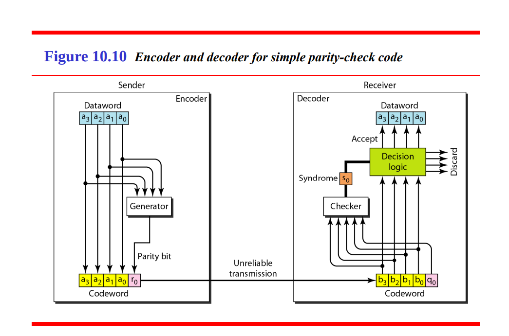
Sender Side (Encoder)
The sender’s role is to encode the data by adding a parity bit to enable error detection at the receiver.
-
Dataword (
a_3, a_2, a_1, a_0):- The dataword is the original 4-bit data to be transmitted:
a_3 a_2 a_1 a_0. - Example:
1011(a_3 = 1, a_2 = 0, a_1 = 1, a_0 = 1).
- The dataword is the original 4-bit data to be transmitted:
-
Generator:
- The generator computes the parity bit
r_0based on the data bits. - How it Works:
- In a simple parity-check code, the parity bit is calculated to ensure the total number of 1s in the codeword (data bits + parity bit) is even (for even parity) or odd (for odd parity).
- The diagram shows the parity bit
r_0being computed as the XOR of the data bits:r_0 = a_3 ⊕ a_2 ⊕ a_1 ⊕ a_0
- XOR Operation:
0 ⊕ 0 = 0,0 ⊕ 1 = 1,1 ⊕ 0 = 1,1 ⊕ 1 = 0.
- This ensures even parity (the number of 1s in
a_3 a_2 a_1 a_0 r_0is even).
- Example:
- Dataword:
1011. - Number of 1s: 3 (odd).
r_0 = 1 ⊕ 0 ⊕ 1 ⊕ 1:1 ⊕ 0 = 11 ⊕ 1 = 00 ⊕ 1 = 1
- So,
r_0 = 1.
- Dataword:
- The generator computes the parity bit
-
Parity Bit (
r_0):- The parity bit
r_0is appended to the dataword to form the codeword. - In this diagram,
r_0is the redundant bit added to the 4-bit dataword, making the codeword 5 bits long.
- The parity bit
-
Codeword (
a_3, a_2, a_1, a_0, r_0):- The codeword is the 5-bit string:
a_3 a_2 a_1 a_0 r_0. - Example: For dataword
1011,r_0 = 1, so the codeword is10111. - Total number of 1s in
10111: 4 (even), which satisfies even parity.
- The codeword is the 5-bit string:
-
Unreliable Transmission:
- The codeword is sent over an unreliable channel, where errors (bit flips) may occur.
- Example: Sent
10111, but received10101(bit 3 flipped from 1 to 0).
Receiver Side (Decoder)
The receiver’s role is to check the received codeword for errors using the parity bit and decide whether to accept the data or discard it.
-
Codeword (
b_3, b_2, b_1, b_0, q_0):- The received codeword is labeled as
b_3 b_2 b_1 b_0 q_0, where:b_3 b_2 b_1 b_0correspond to the received data bits (originallya_3 a_2 a_1 a_0).q_0is the received parity bit (originallyr_0).
- Example: Received
10101(bit 3 flipped):b_3 = 1, b_2 = 0, b_1 = 1, b_0 = 0, q_0 = 1.
- The received codeword is labeled as
-
Checker:
- The checker computes a syndrome to detect errors.
- How it Works:
- The syndrome
s_0is calculated by XORing all bits of the received codeword (data bits + parity bit):s_0 = b_3 ⊕ b_2 ⊕ b_1 ⊕ b_0 ⊕ q_0
- For even parity, if
s_0 = 0, the number of 1s is even → No error (or an even number of errors, which is undetectable). - If
s_0 = 1, the number of 1s is odd → Error detected (e.g., a single-bit error).
- The syndrome
- Example:
- Received:
10101. s_0 = 1 ⊕ 0 ⊕ 1 ⊕ 0 ⊕ 1:1 ⊕ 0 = 11 ⊕ 1 = 00 ⊕ 0 = 00 ⊕ 1 = 1
s_0 = 1→ Error detected (odd number of 1s: 3).
- Received:
-
Syndrome (
s_0):- The syndrome
s_0is the output of the checker. s_0 = 0: No detectable error.s_0 = 1: Error detected (e.g., single-bit error or any odd number of errors).
- The syndrome
-
Decision Logic:
- The decision logic uses the syndrome to determine the action:
- If
s_0 = 0: The codeword is accepted, and the datawordb_3 b_2 b_1 b_0is output as the recovered data. - If
s_0 = 1: The codeword is discarded (indicated by theDoutput), as an error is detected but cannot be corrected with a simple parity-check code.
- If
- Example:
s_0 = 1→ Error detected → Discard the codeword.- In a real system, the receiver might request retransmission (e.g., using ARQ).
- The decision logic uses the syndrome to determine the action:
-
Dataword (
a_3, a_2, a_1, a_0):- If the codeword is accepted (
s_0 = 0), the datawordb_3 b_2 b_1 b_0is output as the recovered data, ideally matching the originala_3 a_2 a_1 a_0. - If discarded, no dataword is output, and further action (e.g., retransmission) may be taken.
- If the codeword is accepted (
How It All Ties Together
- Sender (Encoder):
- Takes a 4-bit dataword
a_3 a_2 a_1 a_0. - Computes the parity bit
r_0using XOR to ensure even parity. - Forms the 5-bit codeword
a_3 a_2 a_1 a_0 r_0and transmits it.
- Takes a 4-bit dataword
- Receiver (Decoder):
- Receives the codeword
b_3 b_2 b_1 b_0 q_0, which may have errors. - Computes the syndrome
s_0by XORing all bits. - Uses the syndrome to decide whether to accept the data (output
b_3 b_2 b_1 b_0) or discard it.
- Receives the codeword
Example Walkthrough
-
Sender:
- Dataword:
1011. - Parity Bit:
r_0 = 1 ⊕ 0 ⊕ 1 ⊕ 1 = 1. - Codeword:
10111. - Number of 1s: 4 (even) → Satisfies even parity.
- Dataword:
-
Unreliable Transmission:
- Sent:
10111. - Received:
10101(bit 3 flipped from 1 to 0).
- Sent:
-
Receiver:
- Received Codeword:
10101. - Syndrome:
s_0 = 1 ⊕ 0 ⊕ 1 ⊕ 0 ⊕ 1 = 1. - Decision:
s_0 = 1→ Error detected → Discard the codeword.
- Received Codeword:
No Error Case:
- Received:
10111(no errors). s_0 = 1 ⊕ 0 ⊕ 1 ⊕ 1 ⊕ 1 = 0.s_0 = 0→ Accept → Output dataword:1011.
Types of Linear Block Codes
-
Hamming Codes:
- Designed for single-bit error correction.
d_min = 3→ Corrects 1 error, detects 2 errors.- Example: (7,4) Hamming Code (as above).
-
Cyclic Codes:
- A subset of linear block codes where a cyclic shift of a codeword is also a codeword.
- Example: CRC (Cyclic Redundancy Check).
- Efficient for burst error detection.
-
Reed-Solomon Codes:
- Linear block codes that operate on symbols (groups of bits).
- Used for correcting multiple errors.
- Applications: CDs, DVDs, QR codes.
Encoder and decoder for a hamming code
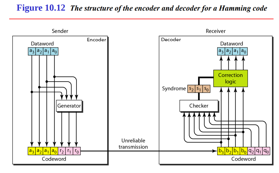
Figure 10.12: The structure of the encoder and decoder for a Hamming code illustrates the encoding and decoding process for a Hamming code, a linear block code designed to correct single-bit errors.
Sender Side (Encoder):
- Dataword (
a_3, a_2, a_1, a_0): The 4-bit input data (e.g.,1011). - Generator: Adds 3 parity bits (
r_2, r_1, r_0) using XOR operations based on specific data bit positions (Hamming code rules).- Example: For
1011, parity bits are computed to form a 7-bit codeworda_3 a_2 a_1 a_0 r_2 r_1 r_0(e.g.,1011010).
- Example: For
- Codeword: The 7-bit output (
a_3 a_2 a_1 a_0 r_2 r_1 r_0) is transmitted over an unreliable channel.
Receiver Side (Decoder):
- Codeword (
b_3, b_2, b_1, b_0, q_2, q_1, q_0): The received 7-bit codeword, which may have errors (e.g.,1010010, bit 4 flipped). - Checker: Computes a 3-bit syndrome (
s_2, s_1, s_0) using XOR operations on specific bit positions.- Example: Syndrome
011(binary 3) indicates an error in bit 4.
- Example: Syndrome
- Correction Logic: Uses the syndrome to locate and correct the error (e.g., flip bit 4:
1010010→1011010). - Dataword (
a_3, a_2, a_1, a_0): Outputs the corrected 4-bit data (e.g.,1011).

Key Points:
- Hamming code corrects single-bit errors (
d_min = 3). - Encoding adds parity bits; decoding uses the syndrome to correct errors.
- Example: Encode
1011→1011010, receive1010010, correct to1011010, output1011.
Burst error correction using Hamming code
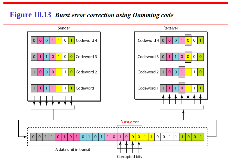
Sender Side:
- Four Hamming codewords (Codeword 1 to 4) are shown, each with 7 bits (e.g., Codeword 1:
1111111, Codeword 2:1100010). - Bits are interleaved column-wise into a single data unit:
- Bit 1 of all codewords:
0111(from Codewords 4, 3, 2, 1). - Bit 2 of all codewords:
0011, and so on.
- Bit 1 of all codewords:
- Resulting data unit:
011100110101...(28 bits total).
Transmission:
- A burst error corrupts 4 consecutive bits in the data unit (highlighted as “Corrupted bits”).
Receiver Side:
- The received data unit is de-interleaved back into the four codewords:
- Codeword 1:
1111011(bit 3 corrupted). - Codeword 2:
1000110(bit 3 corrupted). - Codeword 3:
0110000(bit 3 corrupted). - Codeword 4:
0001001(bit 3 corrupted).
- Codeword 1:
- Each codeword now has only a single-bit error, which a Hamming code (
d_min = 3) can correct. - Hamming decoding corrects each codeword back to its original form (e.g.,
1111011→1111111).
Key Points:
- Interleaving spreads a burst error across multiple codewords, converting it into single-bit errors per codeword.
- Hamming code corrects these single-bit errors, effectively handling the burst error.
Advantages of Linear Block Codes
- Simplicity: Encoding/decoding is efficient using matrix operations.
- Error Handling: Well-defined error detection/correction capabilities based on
d_min. - Hardware-Friendly: Matrix operations (e.g., XOR, AND) are easy to implement in hardware.
- Systematic Form: Easy to extract the original data from the codeword.
Cyclic Codes
A Cyclic Code is a type of linear block code with an additional property: if a codeword is cyclically shifted (i.e., bits are rotated left or right), the result is another valid codeword in the same code. This cyclic property makes them efficient for implementation and particularly good at detecting burst errors.
- Linear: Cyclic codes are linear block codes, meaning the XOR of any two codewords is another valid codeword.
- Block Code: Data is divided into blocks of
kbits, andrredundant bits are added to form ann-bit codeword (n = k + r). - Cyclic: A cyclic shift of any codeword produces another codeword.
Example:
- Code:
{000, 110, 011, 101}. - Codeword:
110. - Cyclic shift (left):
110→101(shift left, move the leftmost bit to the right). 101is also a codeword, confirming the cyclic property.
Key Properties of Cyclic Codes
-
Cyclic Property:
- A cyclic shift of a codeword is another codeword.
- Example: For a 3-bit code, shifting
110to101or011(both directions) must yield valid codewords if the code is cyclic.
-
Linearity:
- As a linear block code, the XOR of any two codewords is another codeword.
- Example:
110 ⊕ 011 = 101, which is also a codeword in the example above.
-
Polynomial Representation:
- Cyclic codes are defined using polynomials over GF(2) (binary field).
- Each
n-bit codewordc_0 c_1 ... c_{n-1}is represented as a polynomial:C(x) = c_0 + c_1x + c_2x^2 + ... + c_{n-1}x^{n-1}
- Example: Codeword
110→C(x) = 1 + 1x + 0x^2 = 1 + x. - Cyclic shift corresponds to polynomial multiplication by
xmodulox^n - 1:- Shift
110to101:C(x) = 1 + x→xC(x) = x + x^2→ Modulox^3 - 1→1 + x^2(which is101).
- Shift
-
Generator Polynomial:
- A cyclic code is generated by a single polynomial
G(x)of degreer = n - k, which dividesx^n - 1. - All codewords are multiples of
G(x)(modulox^n - 1). - Example: For an (n,k) cyclic code,
G(x)has degreer, and codewords are of the formC(x) = M(x) · G(x), whereM(x)is the message polynomial.
- A cyclic code is generated by a single polynomial
-
Minimum Hamming Distance (d_min):
- Determines error-handling capability:
- Detects up to
d_min - 1errors. - Corrects up to
t = floor((d_min - 1)/2)errors.
- Detects up to
- Cyclic codes can be designed with specific
d_min(e.g., CRC has highd_minfor burst error detection).
- Determines error-handling capability:
Structure of Cyclic Codes
Cyclic codes are typically systematic, meaning the codeword contains the original data bits followed by redundant bits.
Polynomial Representation:
- Message Polynomial: A
k-bit messagem_0 m_1 ... m_{k-1}→M(x) = m_0 + m_1x + ... + m_{k-1}x^{k-1}. - Codeword Polynomial: An
n-bit codeword →C(x) = c_0 + c_1x + ... + c_{n-1}x^{n-1}. - Generator Polynomial:
G(x)of degreer = n - k.
Encoding:
- Represent the message as
M(x). - Multiply by
x^rto shift left byrbits (appendrzeros):x^r · M(x). - Divide by
G(x)to get the remainderR(x)(degree <r):x^r · M(x) = Q(x) · G(x) + R(x)
- Codeword:
C(x) = x^r · M(x) - R(x)(in GF(2), subtraction is XOR).- This ensures
C(x)is a multiple ofG(x).
- This ensures
Decoding:
- Use the parity-check matrix or polynomial division to compute the syndrome.
- Syndrome
S(x) = R(x) mod G(x):- If
S(x) = 0, no error. - If
S(x) ≠ 0, an error is detected, and error patterns can be corrected (for error-correcting cyclic codes).
- If
CRC encoder and decoder
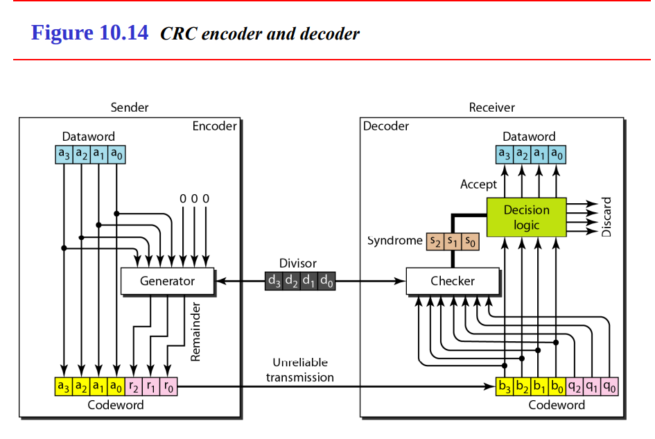
Sender Side (Encoder)
The sender encodes the data by appending a CRC remainder to enable error detection at the receiver.
-
Dataword (
a_3, a_2, a_1, a_0):- The 4-bit input data:
a_3 a_2 a_1 a_0. - Example:
1101.
- The 4-bit input data:
-
Generator:
- The generator computes the CRC remainder using polynomial division (modulo-2).
- Process:
- Append
rzeros to the dataword (whereris the degree of the generator polynomial). - In the diagram,
r = 3(three check bits:r_2, r_1, r_0), so append000. - Example:
1101→1101000. - Divide this by the generator polynomial (represented as the “Divisor”).
- The divisor is typically
G(x)(e.g.,x^3 + x + 1→1011for a degree-3 polynomial). - Division is done using XOR (modulo-2 arithmetic).
- Append
- Example:
- Data:
1101000. - Divisor:
1011. - Divide
1101000by1011→ Remainder =100(d_2 d_1 d_0).
- Data:
-
Remainder (
d_2, d_1, d_0):- The remainder from the division is the CRC (3 bits in this case).
- Example: Remainder
100→r_2 = 1, r_1 = 0, r_0 = 0.
-
Codeword (
a_3, a_2, a_1, a_0, r_2, r_1, r_0):- The codeword is the dataword plus the CRC remainder:
a_3 a_2 a_1 a_0 r_2 r_1 r_0. - Example:
1101+100→1101100. - This codeword is a multiple of the generator polynomial (i.e., divisible by
G(x)with no remainder).
- The codeword is the dataword plus the CRC remainder:
-
Unreliable Transmission:
- The codeword is sent over an unreliable channel, where errors may occur.
- Example: Sent
1101100, received1100100(bit 4 flipped).
Receiver Side (Decoder)
The receiver checks the received codeword for errors using the CRC and decides whether to accept or discard the data.
-
Codeword (
b_3, b_2, b_1, b_0, q_2, q_1, q_0):- The received codeword:
b_3 b_2 b_1 b_0 q_2 q_1 q_0. b_3 b_2 b_1 b_0are the data bits,q_2 q_1 q_0are the received CRC bits.- Example: Received
1100100.
- The received codeword:
-
Checker:
- The checker recomputes the remainder by dividing the received codeword by the same divisor (generator polynomial).
- Process:
- Divide
b_3 b_2 b_1 b_0 q_2 q_1 q_0byG(x)(e.g.,1011). - The result is the syndrome (
s_2 s_1 s_0). - If the syndrome is
000, the codeword is valid (no detectable error). - If the syndrome is non-zero, an error is detected.
- Divide
- Example:
- Received:
1100100. - Divide
1100100by1011→ Remainder ≠ 0 (e.g.,101). - Syndrome:
s_2 s_1 s_0 = 101.
- Received:
-
Syndrome (
s_2, s_1, s_0):- The syndrome indicates whether an error occurred:
s_2 s_1 s_0 = 000: No error (or undetectable error).s_2 s_1 s_0 ≠ 000: Error detected.
- Example:
s_2 s_1 s_0 = 101→ Error detected.
- The syndrome indicates whether an error occurred:
-
Decision Logic:
- Based on the syndrome:
- If
s_2 s_1 s_0 = 000: Accept the codeword, outputb_3 b_2 b_1 b_0as the dataword. - If
s_2 s_1 s_0 ≠ 000: Discard the codeword (indicated by the “Discard” output).
- If
- Example: Syndrome
101→ Discard (error detected). - In a real system, the receiver might request retransmission (e.g., using ARQ).
- Based on the syndrome:
-
Dataword (
a_3, a_2, a_1, a_0):- If accepted, the dataword
b_3 b_2 b_1 b_0is output as the recovered data. - If discarded, no dataword is output.
- If accepted, the dataword
Example Walkthrough
-
Sender:
- Dataword:
1101. - Append Zeros:
1101000. - Divide by
1011: Remainder =100. - Codeword:
1101100.
- Dataword:
-
Transmission:
- Sent:
1101100. - Received:
1100100(bit 4 flipped).
- Sent:
-
Receiver:
- Received Codeword:
1100100. - Divide by
1011: Remainder =101. - Syndrome:
s_2 s_1 s_0 = 101. - Decision: Discard (error detected).
- Received Codeword:
No Error Case:
- Received:
1101100. - Divide by
1011→ Remainder =000. - Syndrome:
000→ Accept → Output dataword:1101.
Encoding Example (CRC as a Cyclic Code)
Consider an (7,4) cyclic code (n = 7, k = 4, r = 3) with G(x) = x^3 + x + 1 (1011).
- Message:
1101→M(x) = x^3 + x^2 + 1. - Shift Left:
x^r · M(x) = x^3 · (x^3 + x^2 + 1) = x^6 + x^5 + x^3.- As bits:
1101000.
- As bits:
- Divide by
G(x):G(x) = x^3 + x + 1(1011).- Divide
1101000by1011(modulo-2):1101000 ÷ 1011→ Remainder =100(R(x) = x^2).
- Codeword:
C(x) = x^r · M(x) - R(x)→1101000 ⊕ 0000100 = 1101100.- Codeword:
1101100(message1101+ check bits100).
Decoding and Error Detection
- Received Codeword:
R(x) = 1100100(bit 4 flipped). - Syndrome:
- Divide
R(x)byG(x):1100100 ÷ 1011→ Remainder ≠ 0 → Error detected.
- Divide
- Correction (if designed for correction):
- Cyclic codes like BCH codes (a subset) can correct errors by mapping syndromes to error patterns.
- For CRC, typically used for detection only, the receiver requests retransmission.
Types of Cyclic Codes
-
Cyclic Redundancy Check (CRC):
- Primarily for error detection.
- High
d_minfor detecting burst errors. - Example: CRC-32 (
G(x) = x^32 + x^26 + ... + 1), used in Ethernet.
-
BCH Codes:
- Cyclic codes designed for multiple error correction.
- Example: A BCH code with
d_min = 5correctsfloor((5-1)/2) = 2errors.
Advantages of Cyclic Codes
- Efficiency: The cyclic property allows encoding/decoding using shift registers (hardware-friendly).
- Burst Error Detection: Excellent for detecting burst errors (e.g., CRC detects all bursts of length ≤ degree of
G(x)). - Algebraic Structure: Polynomial representation simplifies design and analysis.
Limitations
- Error Correction Complexity: While detection is simple (e.g., CRC), correction (e.g., BCH) can be computationally intensive.
- Fixed Length: Like all block codes, they work with fixed block sizes.
- Redundancy Overhead: Adding check bits reduces the effective data rate.
Applications
- CRC: Networking (Ethernet, Wi-Fi), storage (disk drives), file transfer (ZIP files).
- BCH Codes: Satellite communication, memory systems.
Checksum
In computer networks, a checksum is a value used to verify the integrity of data during transmission. It helps detect errors that may have occurred while data was being sent over the network.
Key Points :
- Purpose:
To detect errors in transmitted data. - How it Works:
- The sender calculates a checksum value based on the binary data (usually by summing up segments of the data).
- This checksum is sent along with the data to the receiver.
- The receiver recalculates the checksum from the received data.
- If the recalculated checksum matches the received checksum, the data is considered error-free.
- If not, it means the data was corrupted during transmission.
- Common Methods:
- Internet Checksum (used in protocols like IP, TCP, UDP): Sums up 16-bit words and adds any overflow (carry).
- CRC (Cyclic Redundancy Check): More complex but more accurate; used in Ethernet.
- Limitations:
- Can detect most errors, but not all.
- Cannot correct errors — only detect them.
At the Sender Site:
- Message is divided into 16-bit words
- The data (message) is split into chunks of 16 bits (2 bytes each).
- Checksum word is set to 0
- Before calculating, a placeholder for the checksum is initialized to
0000000000000000.
- Before calculating, a placeholder for the checksum is initialized to
- All words are added using one’s complement addition
- The 16-bit words are added together using one’s complement addition (carry from the MSB is wrapped around to the LSB).
- The sum is complemented → this becomes the checksum
- The final sum is inverted (all bits flipped) to get the checksum.
- Checksum is sent with the data
- This checksum is now attached to the message and sent to the receiver.
At the Receiver Site:
- Message (with checksum) is divided into 16-bit words
- The received message, including the checksum, is split again into 16-bit chunks.
- All words are added using one’s complement addition
- Just like the sender, the receiver adds all the 16-bit chunks including the checksum.
- Sum is complemented to get new checksum
- After adding, the receiver flips the bits of the total sum.
- If the result is 0 → message is valid
- If the final result is all 0s (i.e., 0000000000000000), it means no error.
- If it’s not zero, then the message was corrupted.